

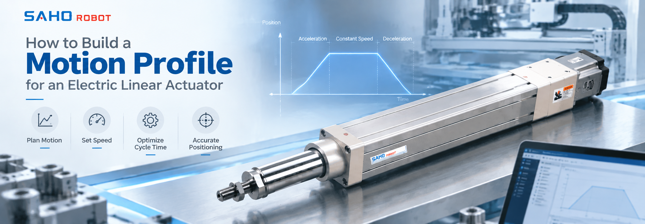
An electric linear actuator motion profile converts a required stroke and machine cycle into the values the axis must actually execute: acceleration, peak or constant velocity, deceleration, and move time. Start with the working stroke, required point-to-point move time, dwell time, return motion, and known controller constraints. Then check whether the move has enough distance for a constant-speed section or becomes triangular. This first-pass calculation defines the kinematic motion profile only; force, motor, thermal, and mechanical sizing remain separate engineering checks. The finished profile should make the complete cycle clear enough for controller validation and actuator engineering review before a final actuator configuration is selected.
Minimum useful output: do not submit only stroke and average speed. Record the stroke, total move time, acceleration time, constant-speed time if present, deceleration time, calculated velocity, dwell, return move, settling time, and repetition rate.
1. Start With the Minimum Inputs and the Complete Machine Cycle
Build the profile from the machine sequence rather than starting with a catalog speed. The first engineering question is: what physical distance must be completed in what amount of time, and what happens immediately before and after that move?
| Input | What to define |
|---|---|
| Working stroke | Required travel for the process move, rather than the complete mechanical travel available. |
| Move time | Time allowed from the start of commanded movement to the required end position. |
| Dwell and settling | Process time while stopped plus any additional time required before the next operation begins. |
| Return motion | Return stroke and return time. Do not assume they are identical to the working move. |
| Application conditions | Payload, moving tooling, mounting orientation, repetition rate, and operating pattern for later engineering review. |
| Controller constraints | Known limits or requirements for velocity, acceleration, deceleration, jerk, and profile generation. |
Break the complete machine cycle into separate time blocks instead of treating it as one average motion:
Cycle time = working move + process dwell + return move + home dwell or settling
A 600 ms working move therefore does not automatically mean a 600 ms machine cycle. Separating the segments also prevents a low average speed from hiding a much higher peak velocity during the actual motion.
Once the required motion is defined, the SEH electric linear actuator page becomes a useful product reference for compact controlled pushing, lifting, or positioning applications. At this stage, however, the objective is still to define the motion requirement—not to select a model from stroke alone.
2. Decide Whether the Move Is Triangular or Trapezoidal
A trapezoidal motion profile contains acceleration, constant velocity, and deceleration. A triangular profile contains only acceleration and deceleration: the axis reaches peak velocity and must immediately begin slowing because there is no remaining distance for a constant-speed segment.
For a first-pass symmetric calculation, let S be stroke, a acceleration, and V the intended velocity. Assume the move begins and ends at zero velocity and uses equal acceleration and deceleration magnitudes. Use one consistent unit system throughout each calculation, such as mm, s, mm/s, and mm/s².
Distance needed to accelerate to V and decelerate to zero:
Sacc+dec = V² / a
| Condition | Profile | Interpretation |
|---|---|---|
| S > V² / a | Trapezoidal | Travel remains after acceleration and before deceleration, so constant-speed motion is possible. |
| S = V² / a | Boundary | Constant-speed time is zero. |
| S < V² / a | Triangular | The intended velocity cannot be reached with the selected acceleration and available stroke. |
For a symmetric triangular move:
Vp = √(a × S)
Ta = √(S / a)
Total move time T = 2 × √(S / a)
This is the practical basis for trapezoidal vs triangular motion profile selection. On short strokes, acceleration and deceleration may consume the complete move, so a velocity entered in the controller should not automatically be treated as an achieved machine velocity.
3. Calculate Acceleration Time, Constant-Speed Time, and Total Move Time
For a symmetric trapezoidal move, let Ta be acceleration time, Tc constant-speed time, and T total move time:
V = a × Ta
T = 2Ta + Tc
S = V(T − Ta)
When stroke and move time are fixed, an engineer can choose an initial acceleration time and calculate the velocity and acceleration needed:
V = S / (T − Ta)
a = V / Ta
Tc = T − 2Ta
If Tc > 0, the profile is trapezoidal. If Tc = 0, it is triangular. If Tc < 0, the selected acceleration time cannot fit inside the required move time.
If acceleration has already been defined, use the smaller physically valid root (0 < Ta ≤ T/2):
Ta = [T − √(T² − 4S/a)] / 2
Feasibility condition: a ≥ 4S / T²
Controller check required: these equations describe first-pass triangular or trapezoidal kinematics. A controller using jerk-limited S-curves, asymmetric ramps, or other motion generation can produce different timing and peak values. Final programmed motion should be verified against the actual controller strategy.
4. Worked Illustrative Example: Build the Profile From Stroke and Move Time
The following numbers are illustrative only. They are not SAHO product specifications, limits, acceptance criteria, or recommended controller settings.
Assume a machine requires a 180 mm working stroke in 0.60 s, with 0.12 s initially allocated to acceleration and 0.12 s to deceleration.
| Parameter | Illustrative value | Calculation |
|---|---|---|
| Working stroke, S | 180 mm | Required travel |
| Move time, T | 0.60 s | Point-to-point target |
| Acceleration time, Ta | 0.12 s | Initial engineering choice |
| Constant-speed time, Tc | 0.36 s | 0.60 − 2 × 0.12 |
| Required velocity, V | 375 mm/s | 180 / (0.60 − 0.12) |
| Acceleration, a | 3,125 mm/s² | 375 / 0.12 |
| Distance per ramp | 22.5 mm | 0.5 × 3,125 × 0.12² |
| Constant-speed distance | 135 mm | 375 × 0.36 |
| Distance check | 180 mm | 22.5 + 135 + 22.5 |
The constant-speed time is positive and the distance calculation closes at 180 mm, so the move is trapezoidal under these assumptions.
Now place it inside an illustrative complete cycle: 0.60 s working move, 0.40 s process dwell, 0.75 s return move, and 0.25 s home dwell or settling. Total cycle time is 2.00 s, equivalent to 30 cycles per minute if the sequence repeats continuously.
Why average velocity is insufficient: the working move averages 300 mm/s, while the calculated constant velocity is 375 mm/s and acceleration is 3,125 mm/s². Those dynamic values belong in the engineering handoff because they describe what the actuator and controller must actually execute.
5. Check Duty Cycle, Settling Time, and Controller Limits Before Release
A mathematically valid profile can still be incomplete as a machine requirement. Before release, review the calculated move against the rest of the cycle and the control strategy.
Do not turn motion-on percentage into a product duty-cycle rating
In the illustrative cycle above, the two moves occupy 1.35 s of the 2.00 s cycle. That ratio describes the sequence only; it is not an allowable actuator duty-cycle specification. Final operating limits depend on the selected actuator, motor and controller, load conditions, orientation, and operating pattern. Engineering confirmation required.
Separate settling from commanded move time
Inspection, dispensing, insertion, or measurement may require the mechanism to become stable after reaching position. Record this as a separate settling requirement. Otherwise, a settling problem can be mistaken for a speed problem and lead to an unnecessarily aggressive motion profile.
Verify the controller profile and return move
Confirm whether the controller uses an ideal trapezoid, automatically changes short moves to triangular profiles, or applies jerk-limited S-curves. If acceleration and deceleration are asymmetric, calculate those segments separately. Treat the return move independently as well when its time, payload condition, or direction differs from the process move.
If the machine architecture is not yet limited to a compact electric actuator, or the project combines several axis types, use the broader guide to plan a complete linear motion solution before committing to one product direction.
6. Prepare the Motion-Profile Data for an Engineering Review
Once the motion calculation is complete, convert it into a short application record. The objective is to let an engineer reconstruct the required movement without interpreting vague descriptions such as “fast return” or “short cycle.”
| Motion and application data to prepare | |
| ✓ Working stroke and direction | ✓ Required working move time |
| ✓ Acceleration / deceleration time | ✓ Calculated peak or constant velocity |
| ✓ Triangular or trapezoidal profile | ✓ Constant-speed time, if present |
| ✓ Dwell and settling time | ✓ Return stroke, time, and profile |
| ✓ Repetition rate / complete cycle | ✓ Payload and moving tooling |
| ✓ Installation orientation and space | ✓ Controller, servo, and jerk constraints |
Multi-stage movement should be submitted as separate segments rather than averaged together. If a machine uses a fast approach followed by a slower process move, record the stroke, velocity, ramp, and time for each stage.
A simple velocity-versus-time sketch is also useful. Mark the acceleration ramp, constant-speed plateau if present, deceleration ramp, dwell, return move, and next cycle. This numerical record and sketch form a much stronger basis for servo sizing and actuator review than a single maximum-speed value.
When does it make sense to continue with the SEH Series?
| Continue to SEH review | The machine requires compact controlled pushing, pulling, lifting, or positioning, and the required stroke, velocity, acceleration, timing, and cycle sequence are now defined. |
| Keep selection open | The machine architecture is still undecided, or the motion is part of a larger transfer or multi-axis system. Review the wider linear-motion solution before fixing the actuator direction. |
| Do not finalize a model yet | Payload, moving tooling, installation direction, controller conditions, available space, or other selection inputs are still missing. Complete the application data and request engineering confirmation. |
Procurement checkpoint: do not compare candidate actuators only by maximum catalog speed. Review whether the selected configuration can execute the required stroke, acceleration, peak velocity, deceleration, cycle frequency, and application conditions together. Final SEH model and configuration selection requires engineering confirmation.
SEH Series Electric Linear Actuator If the motion profile is now defined and the application requires a compact controlled actuator for pushing, pulling, lifting, or positioning, continue to the SEH Series product page to review the available product family. Use the calculated motion data as an engineering input rather than selecting from stroke or top speed alone. 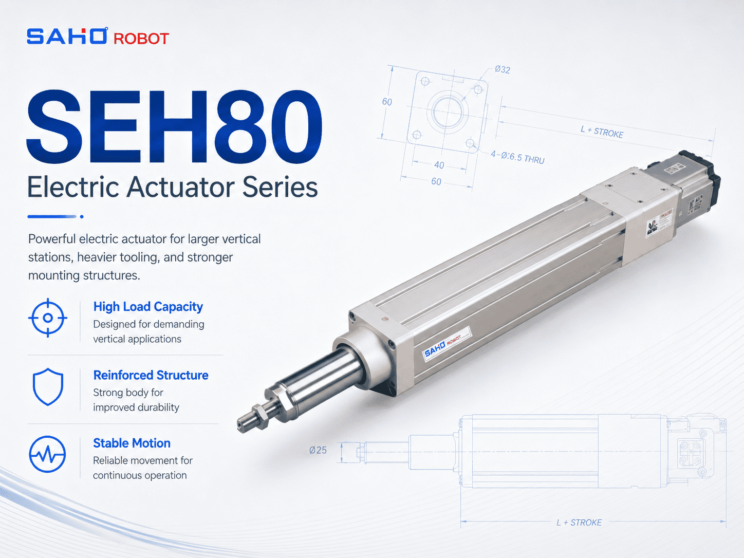 View SEH Series Electric Linear Actuator View SEH Series Product PageBefore final model selection, confirm the complete motion profile together with payload, mounting orientation, available installation space, controller conditions, and other application requirements. |
Frequently Asked Questions About Electric Linear Actuator Motion Profiles
| When does a motion profile become triangular instead of trapezoidal? |
| It becomes triangular when the stroke is too short to reach the intended constant velocity and still decelerate to zero. For symmetric acceleration, compare the available stroke with V²/a. |
| How do dwell time and return motion affect cycle time? |
| Both add directly to the cycle. Calculate the return separately if its speed, acceleration, stroke, direction, or operating condition differs from the working move. |
| Should jerk be included in the first calculation? |
| An ideal triangular or trapezoidal profile is normally sufficient for the first kinematic calculation. If the controller uses jerk-limited S-curves, include jerk during control review because the smoothed ramps can change final timing and peak values. |
| What motion data is needed before selecting an electric linear actuator? |
| Prepare stroke, move time, acceleration and deceleration values or ramp times, peak velocity, dwell, return motion, settling time, repetition rate, payload, mounting orientation, available installation space, and controller constraints. |
Turn the Motion Profile Into an Engineering Review
A useful electric linear actuator motion profile connects the machine cycle to measurable requirements: stroke, move time, acceleration, velocity, deceleration, dwell, return motion, and repetition rate. Once these values are explicit, the next step is not to guess a model number. It is to review the motion profile together with the mechanical and control conditions that affect the final actuator configuration.
Before contacting SAHO: prepare the motion-profile calculation plus payload, moving tooling, installation orientation, available space, controller or servo information, and any special return or settling requirements. This gives engineering a clearer basis for reviewing the application.
Ready to Move From Calculation to Product Review? Review the SEH Series with the completed motion profile, or send the stroke, timing, acceleration, velocity, payload, orientation, and controller information to SAHO for engineering review. Review SEH Series Electric Linear ActuatorContact SAHO for Engineering Review |